4 Bentuk Rumus Excel IF Lengkap dengan Contoh yang Relevan
Letakkan data kedua di kolom lain, misalnya kolom B. Pilih sel kosong di tempat Anda ingin hasil korelasi ditampilkan. Ketikkan rumus =CORREL (A1:A10, B1:B10) di sel tersebut, dengan A1:A10 dan B1:B10 adalah rentetan data yang ingin Anda analisis. Sesuaikan rentetan data dengan jumlah entri yang sesuai.

Cara Membuat Rumus Bulan Di Excel Hongkoong
Fungsi CORREL digunakan untuk menghitung korelasi antara dua rentang data dalam lembar kerja Excel. Korelasi mengukur sejauh mana dua set data bergerak bersamaan. Rumus umumnya adalah sebagai berikut : =CORREL (rentang_data1, rentang_data2) 2. Menentukan Jenis Korelasi. Hasil dari fungsi CORREL adalah nilai antara -1 dan 1.

Rumus Excel yang Perlu Kamu Kuasai, Simak di Sini
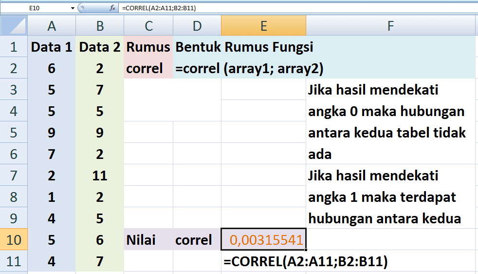
Berikut adalah langkah-langkahnya:1. Siapkan data tinggi badan dan berat badan dalam dua kolom di excel. 2. Ketikkan rumus correl di dalam sel kosong. Contohnya: =CORREL (A2:A11, B2:B11) 3. Tekan Enter pada keyboard. 4. Hasilnya akan muncul di dalam sel yang kamu pilih.
Rumus Dan Contoh Excel Yang Sering Digunakan
The CORREL Function [1] is categorized under Excel Statistical functions. It will calculate the correlation coefficient between two variables. As a financial analyst, the CORREL function is very useful when we want to find the correlation between two variables, e.g., the correlation between a particular stock and a market index.
Cara Menghitung Di Excel Dengan Rumus Warga.Co.Id
The CORREL function returns the correlation coefficient of two cell ranges. Use the correlation coefficient to determine the relationship between two properties. For example, you can examine the relationship between a location's average temperature and the use of air conditioners. Syntax. CORREL(array1, array2)

Rumus And Excel
To draw a correlation graph for the ranked data, here's what you need to do: Calculate the ranks by using the RANK.AVG function as explained in this example. Select two columns with the ranks. Insert an XY scatter chart. For this, click the Scatter chart icon on the Inset tab, in the Chats group.

Cara Membuat Rumus Ranking Di Excel Hongkoong
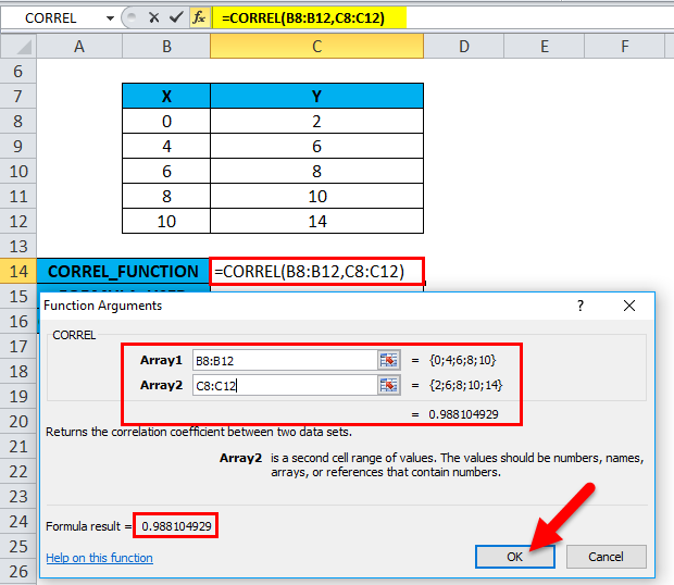
Berdasarkan pada berkas di atas, letakkan kursor pada kolom D12, kemudian ketikkan rumus =CORREL(array1;array2). Array1 adalah seluruh data di kolom X (jam kerja), dan array2 adalah seluruh data di kolom Y (Target) Urutannya, ketikkan rumusnya dulu, =CORREL(, kemudian tandai seluruh data di kolom jam kerja dengan kursor.

Rumus Mencari Nilai Tengah Di Excel Microsoft
Click the Data tab. In the Analysis group, click on the Data Analysis option. In the Data Analysis dialog box that opens up, click on 'Correlation'. Click OK. This will open the Correlation dialog box. For input range, select the three series - including the headers. For 'Grouped by', make sure 'Columns' is selected.
Cara menggunakan rumus microsoft excel
Menggunakan rumus correl di Excel adalah cara mudah dan efektif untuk menganalisis hubungan antara dua variabel. Dengan mengikuti langkah-langkah yang telah dijelaskan di atas, kamu dapat menghitung korelasi dengan mudah dan cepat. Hasil korelasi yang diperoleh dapat membantu kamu dalam membuat keputusan yang lebih baik dan akurat.
Rumus Excel
How to Plot Correlation Graph in Excel. First, select the range of cell C4:D14. Then go to Insert > Insert Scatter and Bubble Plots > Scatter. Then we will see a scatter plot with plot points of Math and Economics. After that we will click on the Plus icon on the side of the chart and then check the Trendline Box.
2 Cara Copy Rumus Pada MS Excel Dengan Cepat dan Mudah
To apply this formula in Excel, follow these four simple steps: Select the cell where you want to display the correlation coefficient. Type '=' sign followed by CORREL (. Select the range of values for the first variable, type a comma, and then select the range of values for the second variable.
Cara Mudah Membuat Rumus Di Excel Untuk Pemula Dengan Contoh Dan LangkahLangkah Tepat Bicara
CORREL di ExcelFungsi CORREL dikategorikan sebagai fungsi statistik di Excel. Rumus CORREL di Excel digunakan untuk mengetahui koefisien korelasi antara dua variabel. Ini mengembalikan koefisien korelasi dari array1 dan array2.Anda dapat menggunakan koefisien korelasi untuk menentukan hubungan antara dua properti.
Cara Menggunakan Rumus Sigma Di Excel
Worksheet Functions. Real Statistics Functions: The Real Statistics Resource Pack contains the following functions where the samples for z, x, and y are contained in the arrays or ranges R, R1, and R2 respectively. CORREL_ADJ(R1, R2) = adjusted correlation coefficient for the data sets defined by ranges R1 and R2.

Cara Membuat Rumus Di Tabel Excel Hongkoong
Rumus Excel Correl (Korelasi) Ketikan pada cell 10 rumus. =CORREL (B4:B9;C4:C9) Sangat simpel dan mudah bukan, hasil nilai korelasi yang didapat sama 0,98. Kriteria untuk mengetahui korelasia atau hubugan sebagai berikut : 0,00 - 0,199 : Hubungan korelasinya sangat lemah. 0,20 - 0,399 : Hubungan korelasinya lemah.
CORREL in Excel (Formula, Examples) How to Use Correlation in Excel?
COVARIANCE.S(R1, R2) = the sample covariance between the data in R1 and R2. CORREL(R1, R2) = the correlation coefficient between the data in R1 and R2. RSQ(R1, R2) = the coefficient of determination between the data in R1 and R2; this is equivalent to the formula =CORREL (R1, R2) ^ 2.

Rumus CORREL Kumpulan Rumus dan Fungsi Excel
With the Data Analysis tools added to your Excel ribbon, you are prepared to run correlation analysis: On the top right corner of the Data tab > Analysis group, click the Data Analysis button. In the Data Analysis dialog box, select Correlation and click OK. In the Correlation box, configure the parameters in this way:
